Parsing Multivalued columns using MOD function

One of the tenets of first normal form database design is to only allow atomic values in a column. However, that is not always the case in the real world.

I recently encountered a multi-valued column on a project and instead of writing a bunch of OR and SUBSTR(right of =) functions, I saw a pattern and used the FIND() [CHARINDEX() in SQL Server] and MOD() [% in SQL Server] functions. The use of the FIND() and MOD() functions was not only easier to maintain (less lines of code) but ran about twice as fast.

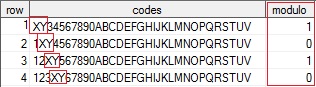
The below code emulates a multi-valued column populated via the SUBSTR(left of) to stuff the 'XY' values in the multi-valued column. The requirement is to find the value 'XY' only on an odd numbered positions (e.g. 1, 3, 5, etc). The FIND() function returns the starting point of the searched string and then the MOD function is used to determine if that position is an odd or even starting location. Modulo finds the remainder after division of one number by another. From Wikipedia:

Given two positive numbers, a (the dividend) and n (the divisor), a modulo n (abbreviated as a mod n) is the remainder of the Euclidean division of a by n. For instance, the expression "5 mod 2" would evaluate to 1 because 5 divided by 2 leaves a quotient of 2 and a remainder of 1, while "9 mod 3" would evaluate to 0 because the division of 9 by 3 has a quotient of 3 and leaves a remainder of 0; there is nothing to subtract from 9 after multiplying 3 times 3.

In order to really see the performance differences in these approaches, I wrote a macro to create a million row SAS data set. After that, the two techniques were bench-marked. The FIND()/MOD() technique took 0.35 seconds vs 0.68 seconds using OR and SUBSTR().

data test( keep = row codes ) ;
  length row 3 codes $32 ;
  do row = 1 to 31 ;
    codes = '1234567890ABCDEFGHIJKLMNOPQRSTUV';
    substr( codes, row, 2 ) = 'XY' ;
    output ;
  end ;
run ;


%macro loopdata ;
  %local setnotes loopdataset ;
  %let setnotes = %sysfunc( getoption( notes ) ) ;
  %let loopdataset = %sysfunc(ceil( %sysevalf( 1000000 / 31 ) ) ) ;
  options nonotes ;  /* turn off notes to the SAS log */
  data testlarge ;
    set
    /* create a millon row data set */
    %do i = 1 %to &loopdataset. ;
      test
    %end ; ;
  run ;
  options &setnotes ;  /* reset NOTES to previous value */
%mend ;
%loopdata

 
proc sql stimer ;
  create table sqlmod as
    select      row
              , codes
              , case
                  when mod( find( codes, 'XY', 'i' ), 2 ) then 1
                  else 0
                end as modulo
      from      testlarge
  ;


  create table sqlsubstr as
    select      row
              , codes
              , case
                  when substr( codes,  1, 2 ) = 'XY'
                    or substr( codes,  3, 2 ) = 'XY'
                    or substr( codes,  5, 2 ) = 'XY'                    
                    or substr( codes,  7, 2 ) = 'XY'
                    or substr( codes,  9, 2 ) = 'XY'
                    or substr( codes, 11, 2 ) = 'XY'
                    or substr( codes, 13, 2 ) = 'XY'
                    or substr( codes, 15, 2 ) = 'XY'
                    or substr( codes, 17, 2 ) = 'XY'
                    or substr( codes, 19, 2 ) = 'XY'
                    or substr( codes, 21, 2 ) = 'XY'
                    or substr( codes, 23, 2 ) = 'XY'
                    or substr( codes, 25, 2 ) = 'XY'
                    or substr( codes, 27, 2 ) = 'XY'
                    or substr( codes, 29, 2 ) = 'XY'
                    or substr( codes, 31, 2 ) = 'XY' then 1
                  else 0
                end as modulo
      from      testlarge
  ;
quit ;

Full width title underline

SAS ODS styles provide opportunities to enhance the appearance of reports. To do this it is required to set an ODS escapechar to establish the inline formatting symbol. I like to use the tilde (~) symbol as in ODS escapechar = "~" ;.

Once the escapechar has been established, use it to set style properties using this syntax "~{style[ property = value ]text to display}" ;.

If you want to have a centered title with a thin red line underneath it spanning the full width of the page, use the width = 100% value (outputwidth= can also be used). The first example below uses the default width= value and is not what was desired. The second attempt works as expected.

options nodate nonumber ;
ods listing close ;
ods escapechar = "~" ;

ods pdf file = "c:\temp\partialline.pdf" ;
  title j = c "~{style[ borderbottmcolor = red 
                        borderbottomwidth = 0.5pt 
                        color = black]SASHELP.CLASS Report}" ;
  proc report data = sashelp.class( obs = 2 ) ;
  run ;
ods pdf close ;


  
ods pdf file = "c:\temp\fullline.pdf" ;
  title j = c "~{style[ borderbottmcolor = red 
                        borderbottomwidth = 0.5pt 
                        width = 100% 
                        color = black]SASHELP.CLASS Report}" ;
  proc report data = sashelp.class( obs = 2 ) ;
  run ;
ods pdf close ;


ods listing ;

UPDATE: 21Dec2015 - from SAS Tech support to create horizontal line across page in ODS PDF:

ODS PDF TEXT = "~{style[ borderbottomcolor = red borderbottomwidth = 0.5pt width = 100%] }" ;

dropColumns Macro

Sometimes you want to remove cluttered columns (i.e. columns where all rows have the same value) from a SAS data set and that is just what the below %dropColumns macro does. Back in 2012 I create a blog post, Drop Missing Columns that handled the removal of NULL values found in either character or numeric columns.

This macro is different in that it handles a single data type at a time, but supports both NULL as well as a fixed value passed as a parameter. So if the following parameters were used, the columns in red below will be removed. The notes in the SAS log that follow will inform you as to what transpired.

    %dropColumns( dsn=x, value=997, type = C )

  NOTE: Dropped 2 of 4 character columns containing "997" from x in 0.040 seconds.
  NOTE: Dropped columns: char1 char2

/**************************************************************************
*     Program: dropColumns.sas
*      Author: Tom Bellmer
*     Created: 03SEP2015 
*     Purpose: drop columns that have the same value in every row.
*       Usage: %dropcolumns( dsn=mydsn, value = 997, type = C )
*       Notes: Use value=, type=C or value=., type=N for NULLs
**************************************************************************/

%macro dropColumns( 
    dsn   =
  , value =
  , type  = C 
) ;

  %local lib mem varlist starttime droplist dropcount ;

  %if not %sysfunc( exist( &dsn. ) ) %then %do ;
    %put %str(E)RROR: The data set &dsn does not exist. ;
    %return ;
  %end ;

  %let type = %upcase( &type. ) ;
  %if &type ne C and &type. ne N %then %do ;
    %put %str(E)RROR: Invalid type = &type. ;
    %return ;
  %end ;

  %let starttime = %sysfunc( datetime() ) ;
  proc sql noprint ;
    %if %index( &dsn., . ) > 0 %then %do ;
      %let lib = %upcase( %scan( &dsn., 1 ) ) ;
      %let mem = %upcase( %scan( &dsn., 2 ) ) ;
    %end ;
    %else %do ;
      %let lib = WORK ;
      %let mem = %upcase( &dsn. ) ;
    %end ;
    select    name
      into    :varlist separated by ' ' 
      from    dictionary.columns
      where       libname = "&lib."
              and memname = "&mem." 
              and type    = ifc( "&type." = "C", "char", "num" ) ;
  quit ;

  %let type = %sysfunc( ifc( &type. = C, $, ) ) ;
  %if &type. = $ %then %let value = %sysfunc( quote( &value. ) ) ;

  data _null_  ;
    length droplist $32767 ;
    set &dsn. end = eof ;

    %if &sqlobs. > 0 %then %do ;
      array avars( * ) &type. &varlist. ;
      array adropvars ( &sqlobs. ) $1 _temporary_ ( &sqlobs. * 'Y' ) ;
      do i = 1 to &sqlobs. ;
        if avars( i ) ne &value. then adropvars( i ) = 'N' ;
      end ;

      if eof then do ;
        do i = 1 to &sqlobs. ;
          if adropvars( i ) = 'Y' then do ;
            dropcount + 1 ;
            droplist = catx( " ", droplist, vname( avars( i ) ) ) ;
          end ;
        end ;
      end ;

      call symputx( 'droplist', droplist, 'l' ) ;
      call symputx( 'dropcount', dropcount, 'l' ) ;
    %end ;
  run ;

  %if %symexist( dropcount )  %then %do ;
    data &dsn ;
      set &dsn( drop = &droplist ) ;
    run ;

    %put NOTE: Dropped &dropcount of %sysfunc( countw( &varlist. ) ) %sysfunc(ifc(&type=$,character,numeric)) columns containing &value. from &dsn. in %sysfunc( strip( %sysfunc( putn( %sysevalf( %sysfunc( datetime()) - &starttime.),9.3) ) ) ) seconds. ;
    %if &dropcount > 0 %then %do ;
      %put NOTE: Dropped columns: &droplist. ;
    %end ;
  %end ;
  %else %do ;
    %put NOTE: no columns were dropped. ;
  %end ;
%mend ;

/* EOF: dropColumns.sas  */

Column Splitter Take 2 - Merge

An anonymous person provided an alternative take on my %columnSplitter macro and I have to admit this one is easier to understand, has less code and runs about twice as fast. Congrats to whomever shared this alternative approach.

Here is the complete code using the merge statement:

%macro columnSplitter2( 
    columns = 3
  , indsn   =
  , outdsn  =
  , varname =  
) ;
 
  %local dsid nobs increment ;

  %if not %sysfunc( exist( &indsn. ) ) %then %do ;
    %put %str(E)RROR: invalid input data set name: &indsn. ;
    %return ;
  %end ;

  %if %isblank( &indsn. ) %then %do ;
    %put %str(E)RROR: invalid output data set name: &outdsn. ;
    %return ;
  %end ;

  %if %isblank( &varname. ) %then %do ;
    %put %str(E)RROR: invalid variable name: &varname. ;
    %return ;
  %end ;

  %let dsid      = %sysfunc( open( &indsn. ) ) ;
  %let nobs      = %sysfunc( attrn( &dsid., nobs ) ) ;
  %let dsid      = %sysfunc( close( &dsid. ) ) ;
  %let increment = %sysfunc( ceil( &nobs. / &columns. ) ) ;

  data &outdsn. ;
    merge
    %do i = 1 %to &columns ;
      &indsn( 
        keep     = &varname 
        rename   = ( &varname = &varname&i ) 
        firstobs = %eval( ( &i. - 1 ) * &increment. + 1 ) 
        obs      = %eval( &i. * &increment. ) )
    %end ;
    ;
  run ;

%mend ;

%columnSplitter2(columns=3,indsn=states,outdsn=statessplit3,varname=statename)

Column Splitter

I created a report that includes a one page table of contents. Having a single column of all 50 states runs off the page, so I wanted to create additional columns to spread the data horizontally. The %columnSplitter() macro was created to support this capability.

In the below code, several SAS Component Language (SCL) functions are used to process the data. The OPEN() function supports reading data sets in random access instead of sequential access mode. The dsid variable is a pointer to the data set and can be used with many other functions to determine data types, length and number of rows. The %isblank macro code can be found here.

An ARRAY is used to assign the number of columns to create. That value must be determined at compile time, hence the need for the DATA _NULL_ step prior to the assignment of the array subscript. The offset variable is the result by dividing the total number of logical rows by the desired number of columns. The key to the program is the use of the FETCHOBS() function to read a specified row number.

Based on the data type of the &varname variable, a getvarc()/getvarn() function is used to obtain the value of that row. After data for all columns is collected and output, the call missing( of colname[*] ) function is used to reset all array elements to missing. Finally, what gets opened must be closed using the CLOSE() function.

data states ;
  do statecode = 1 to 56 ;
    statename = fipnamel( statecode ) ;
    if statename not in ('Invalid Code', 'District of Columbia' ) then output ;
  end ;
run ;

%macro columnSplitter( 
    columns = 3
  , indsn   =
  , outdsn  =
  , varname =  
) ;

  %local length vartype varnum i j k ;

  %if not %sysfunc( exist( &indsn. ) ) %then %do ;
    %put %str(E)RROR: invalid input data set name: &indsn. ;
    %return ;
  %end ;

  %if %isblank( &indsn. ) %then %do ;
    %put %str(E)RROR: invalid output data set name: &outdsn. ;
    %return ;
  %end ;

  %if %isblank( &varname. ) %then %do ;
    %put %str(E)RROR: invalid variable name: &varname. ;
    %return ;
  %end ;

  data _null_ ;
    dsid = open( "&indsn." ) ;
    varnum = varnum( dsid, "&varname." ) ;
    call symputx( 'varnum', varnum ) ;
    vartype = vartype( dsid, varnum ) ;
    call symputx( 'vartype', vartype ) ;
    call symputx('length',cats(ifc(vartype='C','$',''),varlen(dsid,varnum)));
    dsid = close( dsid ) ;
  run ;

  data &outdsn. ( keep = colname: ) ; 
    array colname[ &columns. ] &length. ; 
    dsid = open( "&indsn." ) ;
    totalobs = attrn( dsid, 'nlobs' ) ;
    offset = ceil( totalobs / &columns. ) ;
    do i = 1 to offset ;
      k = 1 ;
      do j = 0 by offset while( k <= &columns. ) ;
        rc = fetchobs( dsid, i + j ) ;
        if ( i + j ) <= totalobs then do ;
          if "&vartype." = "C" then colname[k] = getvarc(dsid, &varnum.) ;
          else colname[ k ] = getvarn( dsid, &varnum. ) ;
        end ;
        k + 1 ;
      end ;
      output ;
      call missing( of colname[ * ] ) ;
    end ;

    dsid = close( dsid ) ;
    stop ;
  run ;
%mend ;

%columnSplitter(columns=3,indsn=states,outdsn=statessplit3,varname=statename)
%columnSplitter(columns=4,indsn=states,outdsn=statessplit4,varname=statename)

The Tooth about Tobacco

If after reading Robert Allison's and Rick Wicklin's SAS blog posts on toothlessness you're saying "Yeah baby!, Yeah!" I want to read more, then you have come to the right place.

No one wants to lose their teeth, yet there is good chance this will happen to many people once they become senior citizens. One of the things in Rick's post was a correlation between median income in a state and the number of edentulous individuals. When I ran a proc corr against the data he provided, the relationship was -0.63442. Not bad, but I wondered if other variables were more highly correlated to toothlessness.

I wondered if instead of income, Body Mass Indicator or BMI might be more highly correlated to one losing teeth. Sure enough, as the below code and graph reveals, the correlation increased to 0.73565 using BMI as a variable.

data teethcig ;
  merge teeth cigs ;
  by state ;
run ;

proc corr 
  data = teethbmi 
  noprint 
  outp = opbmi( where = ( _type_ = 'CORR' and _name_ = 'BMI' ) )  ;
  var bmi pct ;
run ;

data _null_ ;
  set opbmi ;
  call symputx( 'BMICORR', put( pct, 8.5 ) ) ;
run ;

title "All Teeth Extracted vs. BMI";
footnote j = l "Source: http://www.cdc.gov/obesity/data/table-adults.html" ;
proc sgplot data = teethbmi ;
  scatter x = bmi y = pct / datalabel = state ;
  loess   x = bmi y = pct ;
  refline 18.5 / 
    axis = x 
    label = "Normal (18.5 - 24.99)"   
    lineattrs = ( color = red ) ;
  refline 25 / 
    axis = x 
    label = "Overweight (25 - 29.99)" 
    lineattrs = ( color = red ) ;
  refline 30 / 
    axis = x 
    label = "Obese (over 30)" 
    lineattrs = ( color = red ) ;
  xaxis values = ( 17.5 to 37.5 by 2.5 ) ;
  inset "Correlation Coefficient = &bmicorr" / 
    border 
    title = "Pearson" 
    position = bottomright ;
run ;

After looking at the output, I started to wonder if another variable such as tobacco usage might be more highly correlated to tooth loss than BMI. I was surprised to discover that the overall median adult cigarette smoking prevalence across states was 21.2% in 2011 using data provided by the Center for Disease Control or CDC. When cigarette smoking was correlated to toothlessness by state, the pearson correlation coefficient increased to 0.77286 as can be seen in the next graph.

Taking into consideration the usual caveat that correlation does not imply causation, if you want to retain your teeth it is likely best to avoid smoking, eat well, make more money and brush those chompers...

The full source code can be found here.

Updating an ODS tagset

Chevell Parker has written a few excellent papers on the TAGSETS.TABLEEDITOR tagset that can be found here, here and here. ODS TAGSETS such as TABLEEDITOR are saved as item stores and need to be updated as the code can change over time. I do not update tagsets often, so created this blog entry for future reference and to share with others looking to do the same.

You can see the templates that are available by issuing the ODS PATH SHOW command. Individual tagsets in a library can be seen using SAS display manager by clicking on the Explorer window then at the bottom click on the Results tab. After that, left-mouse click on the Results node then Templates. Alternatively, you could issues ODSTEMPLATES in the SAS command window.

In the case of the TAGSETS.TABLEEDITOR I wanted to know the date and version that I was using. That can be achieved by adding OPTIONS( doc = "quick" ).

See the below code for the steps I used to update the tagset. You can also refer to Usage Note 32394: Installing and Storing Updated Tagsets for ODS MARKUP.

  libname common "pathgoeshere" ;

  ods path show ;
      current ODS PATH is:
      1. COMMON.TEMPLAT(READ)
      2. SASUSER.TEMPLAT(UDPATE)
      3. SASHELP.TMPLMST(READ)

  ods tagsets.tableeditor 
    file = "c:\temp\junk.html" 
    options( doc = "quick" ) ;
  ods tagsets.tableeditor close ;
      NOTE: Writing TAGSETS.TABLEEDITOR body file: c:\temp\junk.html
      v2.65  4/25/2013

  *-- set the template mode from READ to UPDATE ;
  ods path common.templat(update) ;

  filename temp url 
   'http://support.sas.com/rnd/base/ods/odsmarkup/tabeleditor/tableeditor.tpl';
  %inc temp ;
     NOTE: Overwritting existing template/link: Tagsets.Tableeditor
     NOTE: TAGSET 'Tagsets.Tableeditor' has been save to: COMMON.TEMPLAT
  filename temp clear ;

  ods path reset ;
  ods path show ;
     Current ODS PATH list is:
     1. SASUSER.TEMPLAT(UPDATE)
     2. SASHELP.TMPLMST(READ)

  *-- reset common.templat as the first to be read in READ mode ;
  ods path(prepend) common.templat(read) ;
  ods path show ;
      current ODS PATH is:
      1. COMMON.TEMPLAT(READ)
      2. SASUSER.TEMPLAT(UDPATE)
      3. SASHELP.TMPLMST(READ)

  *-- show that the tagset has been updated as it has ;
  ods tagsets.tableeditor 
    file = "c:\temp\junk.html" 
    options( doc = "quick" ) ;
  ods tagsets.tableeditor close ;
      NOTE: Writing TAGSETS.TABLEEDITOR body file: c:\temp\junk.html
      v3.14  3/2/2015  

Four Short Macro Functions

SAS macro functions are very useful routines to return a value like a regular SAS or custom function created by proc fcmp. This blog entry contains a collection of four short, simple and to the point macro functions that you may find of some value.

In his paper, "Is This Macro Parameter Blank" Chang Y Chung does a great job testing ways to determine if a macro variable is blank. The most solid way to do this is as follows:

  %macro isBlank( param ) ;
    %sysevalf( %superq( param ) =, boolean )
  %mend ;

The idea for the next function was obtained from Art Capenter's paper which returns the name of the SAS program being executed. It is important to test for SYSIN value first as that is how you get the program name from a batch invocation.

  %macro pgmname() ;
    %local retval ;
    %let retval = %sysfunc( getoption( sysin ) ) ; /* batch mode */
    %if %isblank( &retval. ) %then 
      %let retval = %sysget( sas_execfilepath ) ; /* interactive mode */
    &retval.
  %mend ;

SAS veteran, Peter Crawford was a featured presenter a SAS Global Forum 2015. I really liked his %now function to return the time, day of week and date using the TWMDY format. You can see his video here: Learn Hidden Ideas in Base SAS® to Impress Colleagues

  %macro now( fmt = twmdy. ) / des = 'timestamp' ;
    %sysfunc( strip( %sysfunc( datetime(), &fmt ) ) ) 
  %mend ;

The final short macro function is one I created to obtain attributes from a SAS data set. It can handle character or numeric return values by testing the value of the attribute to return. This macro utilizes the ATTRC and ATTRN functions.

  %macro getattr( dsn =, attr = nobs ) ;
    %local attrtype clist dsid retval ;
    %if %isblank( &dsn ) %then %do ;
      %put %str(E)RROR: the DSN value is missing ;
      %return ;
    %end ;

    %let retval = . ;

    %let clist = CHARSET ENCRYPT ENGINE LABEL LIB MEM MODE 
                 MTYPE SORTEDBY SORTLVL SORTSEQ TYPE ;

    %if %index( &clist., %upcase( &attr. ) ) %then %let attrtype = attrc ;
    %else %let attrtype = attrn ;

    %let dsid = %sysfunc( open( &dsn. ) ) ;
    %if &dsid. %then %do ;
      %let retval = %sysfunc( &attrtype.( &dsid., &attr. ) ) ;
      %let dsid = %sysfunc( close( &dsid. ) ) ;
    %end ;

    &retval. 
  %mend ;

Putting it all together in a program looks like this:

  data values ;
    length name value $64 ;
    name = "Program Name:" ;
    value = "%pgmname()" ;
    output ;
    name = "Now:" ;
    value = "%now()" ;
    output ;
    name = "Engine:" ;
    value = "%getattr( dsn = sashelp.class, attr=engine )" ;
    output ;
    name = "Obs:" ;
    value = "%getattr( dsn = sashelp.class )" ;
    output ;
  run ;

Reading multiple CSV files containing a header row

SAS allows you to read in multiple files with a wildcard which works out great for files that do not contain a header row. The firstobs = 2 can be used on a single file being processed but that only works on the first file of a concatenated set of files to be processed.

The way to get around this limitation is to use the EOV=variable option on the INFILE statement. It is important to understand that EOV is set to 1 when it encounters the first row of the 2nd and subsequent files. However, EOV stays set to 1 so you need to reset it to 0 in your code. Also the EOV=variable is treated as an automatic variable such as _N_ and _ERROR_ and it not written to the data set.

The below code uses prior blog entries split DSN to CSV and delete external files using wildcards in the creation of the sample code. The key to testing for the first row of a new file is the trailing @ on the input @ line. If that sets EOV = 1 then EOV is reset to 0 and the row is deleted. Otherwise that row is re-read on the next input statement.

%splitdsntocsv( 
    dsn          = sashelp.class
  , byvar        = sex
  , outputprefix = c:\temp\temp_
  , outputsuffix = csv
  , header       = Y )

filename fileref 'c:\temp\temp_*.csv' ;
data class2 ;
  infile fileref
    dsd
    truncover
    firstobs = 2 
    eov      = eov ;

  input @ ;

  if eov then do ;
    /* EOV = 1 after first row of next file and needs to be reset to 0 */
    eov = 0 ;
    delete ;
  end ;

  input name $ sex $ age height weight ;
run ;
filename fileref clear ;

%deletefiles( filename = c:\temp\temp_?.csv )

split DSN to CSV

The below macro can be used to split a SAS data set into comma separated value (CSV) files based on the &byvar macro variable. The macro parameters support the option of including or ignoring the header row.

After some initial parameter verification, the dictionary.columns table is used to obtain the name of columns in the correct order. The input data set is then sorted on the &byvar macro variable to a new temp_&memname data set.

A data _NULL_ (do not create a SAS data set) step creates the output files via the use of the filevar= option. The filevar=variable (character string containing the physical filename) is used to dynamically specify the file used by the put statement. Interestingly, the filevar = variable is not written to the output file rather it is treated like other SAS automatic variables such as _N_ or _ERROR_.

The delimiter sensitive data (DSD) option uses a comma ( , ) as the default delimiter, so there is no need to specify a DLM= value. The put ( _ALL_ ) ( : ) is a formatted output statement [syntax is ( var list ) ( format list )] that writes out all non automatic variables to the output file. You could add the _N_ automatic variable such as put ( _N_ _ALL_ ) ( : ) if you wanted to show the row number. Just be sure to also alter the header and understand that _N_ does not get reset to zero when changing by groups. The last step is to clean up (delete) the temporary data set via proc delete.

%macro splitdsntocsv
  ( 
      dsn          = sashelp.class
    , byvar        = sex
    , outputprefix = c:\temp\temp_
    , outputsuffix = csv
    , header       = Y 
  ) ;

  %local libname memname names ;

  %if %sysfunc( exist( &dsn. ) ) = 0 %then %do ;
    %put %str(E)RROR: the DSN = &dsn. does not exist. ;
    %return ;
  %end ;

  %if &byvar. = %then %do ;
    %put %str(E)RROR: the BYVAR = macro variable was not supplied. ;
    %return ;
  %end ;

  %let header = %upcase( %substr( &header., 1, 1 ) ) ;

  %if %index( &dsn., . ) %then %do ;
    %let libname = %scan( &dsn., 1 ) ;
    %let memname = %scan( &dsn., 2 ) ;
  %end ;
  %else %do ;
    %let libname = work ;
    %let memname = &dsn. ;
  %end ;

  proc sql noprint ;
    select         name
      into         :names separated by ","
      from         dictionary.columns
      where            libname = "%upcase( &libname. )"
                   and memname = "%upcase( &memname. )"
      order by     varnum ;     

    %if not %sysfunc( find( "&names.", &byvar., i ) ) %then %do ;
      %put %str(E)RROR: The BYVAR = &byvar. does not exist. ;
      quit ;
      %return ;
    %end ; 

    create table temp_&memname. as
      select       *
        from       &dsn.
        order by   &byvar. ;
  quit ;

  data _null_  ;
    set temp_&memname. ;
      by &byvar. ;
         
    temp_var = cats( "&outputprefix.", &byvar., ".", "&outputsuffix." ) ;
    file tempfref dsd lrecl = 32767 filevar = temp_var ;

    if first.&byvar. and "&header." = "Y" then put "&names." ;
    put ( _all_ ) ( : ) ;
  run ;

  proc delete data = temp_&memname. ;
  run ;
%mend ;

Delete External Files using Wildcards

In the age of cloud computing you may not know the operating system (OS) that SAS is using. As a result, it is best to use SAS functions and statements that are OS independent.

SAS functions are used in the below code to delete one or multiple external files via DOS like wildcard characters. This means that the question mark (?) represents a single character while an asterisk (*) is used for one or more characters. However, those DOS wildcard symbols do not directly translate, so Perl Regular Expression (PRX) functions included in the base SAS language are used.

The FINDC() function is used to find the last slash (\ used by Windows) or backslash (/ used by Linux/UNIX). FINDC() will look for either the / or \ character starting from the end of the string via the -9999 parameter. Once the file portion of the &filename macro variable has been parsed, the TRANWRD function is used to substitute the correct Perl Regular Expression (PRX) characters. PRX reserves the period (.) to represent character so it needs to be escaped (\) as in \. to find a literal period. The entire regular expression is enclosed between the /^ (match beginning of string) to /i (case insensitive)

From there the path or folder is opened using the DOPEN function. The number of entries in the folder are determined by the DNUM function and then the filenames in the folder are read using the DREAD function. After that, the PRXMATCH function is used to determine if the file matches the supplied pattern. Files that match the pattern are then verified with FEXIST and deleted using the FDELETE function.

Here are a few examples of how this can be used followed by the source code:

%deletefiles( filename = c:\temp\xyz.csv ) /* single file */
%deletefiles( filename = c:\temp\xy?.csv ) /* ? for single character */
%deletefiles( filename = c:\temp\x*.csv ) /* files with X ends with .CSV */

%macro deletefiles( filename = ) ;
  %if %sysevalf( %superq( filename ) =,  boolean ) %then %do ;
    %put %str(E)RROR: filename was not supplied.;
    %return ;
  %end ;

  data _null_ ;
    length 
      path file name fullfilename prxstring $256 
      dir filep $8 
      rc did i cnt 4 ;

    path      = substr( "&filename.", 1, findc( "&filename", "\/", -9999 ) ) ;
    file      = substr( "&filename.", findc( "&filename", "\/", -9999 ) + 1 ) ;
    prxstring = cats( "/^"
              , tranwrd(tranwrd(tranwrd(file,".", "\."),"*",".*" ),"?",".?")
              , "/i" ) ;
    
    rc = filename( dir, path ) ;
    if rc = 0 then do ;
      did = dopen( dir ) ;
 
      if did > 0 then do ;
        do i = 1 to dnum( did ) ;
          name = dread( did, i ) ;

          if prxmatch( prxstring, name ) then do ;
            fullfilename = cats( path, name ) ;
            rc = filename( filep, fullfilename ) ;
            if rc = 0 and fexist( filep ) then do ;
              rc = fdelete( filep ) ;
              if rc = 0 then put "NOTE: " fullfilename "has been deleted." ;
              cnt + 1 ;
            end ;
            rc = filename( filep, " " ) ;
          end ;
         
        end ;
        rc = dclose( did ) ;
      end ;
      
      rc = filename( dir, " " ) ;
    end ;
    put / "NOTE: " cnt "files were deleted." ;

   run;
%mend ;
 

Custom inclusive ranges using proc univariate

Using the LEVELS= option in proc gmap makes it easy to split data into equally distributed segments. However, there are times when the results are not exactly what you desire.

This is where the use of proc univariate can help get you most of the way there. The trick is to get the value that is just before the maximum value to display an inclusive range. You can use the SEXCL and/or EEXCL options in proc format but I wanted the legend to show the distinct unambiguous ranges.

Once completed, you can just change the levels = to discrete and use a custom format. The below code shows how this can be achived.

data sampledata ;
  format value comma8.2 ;
  do _n_ = 1 to 1000 ;
    value = round( ranuni( 1 ) * 10000, .01 ) ;
    output ;
  end ;
run ;

proc sort data = sampledata ;
  by value ;
run ;

proc univariate 
  data = sampledata
  noprint ;

  var value ;
  format _numeric_ comma8.2 ;

  output 
    out = univariate
    pctlpts  = 0 to 100 by 20  
    pctlpre = p_ ;
run ;



proc transpose 
  data = univariate 
  out  = ranges
         ( 
            rename = 
              ( 
                _name_ = range 
                col1   = boundary 
               ) 
            drop = _label_ 
         )  ;
run ;



data maxless1( drop = value ) ;
  set ranges ;
  format previousvalue comma8.2 ;

  do while( value < boundary ) ;
    previousvalue = value ;
    set sampledata ;
  end ;

  output ;
run ;



data formatdata( keep = fmtname start end label type ) ;
  retain 
    fmtname 'unirange' 
    type 'n' ;

  set maxless1 end = eof ;

  start = lag( boundary ) ;
  end = previousvalue ;
  if eof then end = boundary ;
  label = catx( " - ", put( start, comma8.2 ) , put( end, comma8.2 ) ) ;
  if _n_ > 1 then output ;
  format start end comma8.2 ;
run ;



proc format 
  lib    = work 
  cntlin = formatdata ;
run ;

proc freq 
  data = sampledata ;

  table value ;
  format value unirange. ;
run ;

Shapefile Import and Census Maps

Click for larger image

I was inspired to write this blog entry after reading the article Here are the fastest growing and fastest shrinking counties in the US by Andy Kiersz. Because I am using SAS 9.2 TS2M3, the maps.uscounty data set does not reflect all county FIPS codes thus requiring creation of my own version from a shapefile. The missing county FIPS values can be identified here. Starting in version 9.3, SAS started using Gfk map data sets that are up to date and do reflect the counties missing in traditional map data sets.

The first step in the SAS program (see below) is to use an URL access method to directly read in the county level data from the Census web site. After that, I used proc mapimport to convert a shapefile to a SAS map data set. Because I only wanted to show the 50 states, FIPS defined territories were removed from the imported data.

The imported data is written to separate data sets for the 48 contiguous states, Alaska and Hawaii. After that, each of those data sets are projected for proper display on a map. Alaska is reduced in size by 60% and then both Alaska and Hawaii are repositioned under the southwestern states. Finally all projected data sets are combined together and then sorted by state.

Proc gremove is used to get the state outlines and then use the annotate facility to draw thicker state outlines. Annotation is also used to write values to the center of each state.

A framed shadowed legend is created and positioned to the right of the map output. I utilized a technique learned from SAS/Graph expert, Robert Allison, to create a blank -90 degree angled title to allow space for the legend.

The last step is to create choropleth maps using proc gmap. Both the state and county output use the same color patterns and levels (10). You can see the full PDF version of the output here.

%macro populationchange ;
  %local states statescount i colors colorscount ;
  %let states = states48 alaska hawaii ;
  %let statescount = %sysfunc( countw( &states. ) ) ;
  %let colors = cb0020 df4949 ef9277 f5c0a9 f6e4dd 
                e0ebf1 b3d5e6 82bbd8 4196c7 0471b0 ;
  %let colorscount = %sysfunc( countw( &colors. ) ) ;

  filename census url 
  "http://www.census.gov/popest/data/counties/totals/2014/files/CO-EST2014-alldata.csv" ;
  data statedata countydata ;
    length state county 5  ;
    infile census dsd dlm = "," truncover firstobs = 2 ;
    input sumlev region division state county stname $ ctyname : $32. 
          pop10 estb10 pest10 pet11 pest12 pest13 pest14 ;
    pctchg = ( ( pest14 - pest13 ) / pest13 ) ;
    format pctchg percent8.2 ;
    if county = 0 then output statedata ;
    else output countydata ;
    keep state county pctchg ;
  run ;
  filename census clear ;

  proc mapimport datafile = 'c:\temp\cb\cb_2013_us_county_500k.shp' 
    out = shapefile ;
    select geoid ;
  run ;

  data alaska hawaii states48 ;
    length state county 5 ;
    set shapefile ;
    where segment < 3 and not missing( x ) ;

    state = input( substr( geoid, 1, 2 ), 2. ) ;
    if state > 56 or state in ( 7, 14, 43, 52 ) then delete ;
    county = input( substr( geoid, 3, 3 ), 3. ) ;

    if sign( x ) = 1 then x = -x ;
         if state =  2 then output alaska;
    else if state = 15 then output hawaii ;
    else                    output states48 ;
    drop geoid ;
  run ;

  %do i = 1 %to &statescount. ;
    /* Project each map data set separately. */
    proc gproject data = %scan( &states., &i. ) 
      out  = projected%scan( &states., &i. )
      eastlong deg ;
      id state county ;
    run;
  %end ;

  data projectedalaska ;
    set projectedalaska ;
    x = ( x * .4 ) - .29629586 ;
    y = ( y * .4 ) - .142574262 ;
  run ;

  data projectedhawaii ;
    set projectedhawaii ;
    x = x -.31 ;
    y = y - .120521998 ;
    if x > -.3726 ;
  run ;

  %do i = 2 %to &statescount. ;
    proc append base=projectedstates48 data=projected%scan( &states., &i. ) ;
    run ;
  %end ;

  proc sort data = projectedstates48 out = counties ;
    by state ;
  run ;

  proc gremove data = counties out = states( where = ( segment <= 8 ) ) ;
    id county ;
    by state ;
  run ;

  data countiesoutline ;
    retain xsys ysys '2' when 'a' color 'black' size 2 style 'empty' ;
    length function $8 ;

    set states ;
      by state segment ;
    if first.state or first.segment then function = 'poly' ;
    else function = 'polycont' ;
  run ;

  data mapanno2 ;
    length function $8 text $16 size 8 ;
    retain xsys ysys '2' hsys '3' when 'a' style "'Albany AMT'" ;

    merge
      statedata  
      maps.uscenter( where = ( fipstate( state ) ne 'PR' ) ) ;
        by state ;

    text = catx( " / ", fipstate(state), strip(putn(pctchg,'percent7.2'))) ;
    lagocean = lag( ocean ) ;
    size = 1.5 ;

    if ocean = 'Y' then do ;
      function = 'label' ;
      position = '6' ;
      output ;
      function = 'move' ;
      output ;
    end ;

    position = '5' ;
    if ocean = 'N' then do ;
      if lagocean = 'Y' then do ;
        function = 'draw' ;
        size = round( 1.5 / 4, .01 ) ;
      end ;
      else do ;
        function = 'label' ;
        position = '2' ;
        text = fipstate( state ) ;
        output ;
        position = '5' ;
        text = putn( pctchg, 'percent7.2' )  ;
      end ;
    end ;
    output ;
  run ;

  options nodate nonumber orientation = landscape ;
  %do i = 1 %to &colorscount. ;
    pattern&i. v = s c = cx%scan( &colors., &i. ) ;
  %end ;
  legend1 position = right across = 1 mode = share
    label = ( position = top font = "albany amt/bold" j = c 'Percent Change' ) 
    shape = bar( .12in, .12in ) cshadow = gray 
    offset = ( 2, 3 ) frame ;
 
  title1 h = 3 "2013 to 2014 Population Change";
  title5 a = -90 h = 4pct " ";
  footnote j=l "Source: US Census Bureau, 2014 Population Estimates" ;

  ods listing close ;
  ods pdf file = 'c:\temp\populationchange.pdf' notoc ;
    proc gmap data = statedata 
      map = maps.us( where = ( fipstate( state ) ne 'PR' ) ) all ;
      id state ;
      choro pctchg / anno = mapanno2 legend = legend1 levels = &colorscount. ;
    run ;
    
    proc gmap data = countydata map = counties all ;
      id state county ;
      choro pctchg / anno = countiesoutline legend = legend1  
        levels = &colorscount.  ;
    run ;
    quit ;
  ods pdf close ;
  ods listing ;
%mend ;
%populationchange

Data Driven Report using the VVALUEX function

The SAS VVALUEX function can be used to display the contents of a variable based on another variable. VVALUEX is somewhat similar to a SAS macro variable but it will create a 200 byte character variable unless the variable has been previously defined with a length or attrib statement. This really comes into play when data driving a program to change a column's format or conditionally display an image as is done here. Be sure to click on the images to see larger versions.

The cardata data set contains raw data collected from various sources on the fastest automobile for each of the Big 3 auto makers. The below image reveals the contents of this data set.

The carmetadata table is used to define the label and format to be used along with the name of the variable to be resolved. A tilde (~) is being used as the ODS escapechar - adding the underscore (_) simulates a non breaking space which is how the 4 character indentation works. Here is what that looks like:

A data step is used to read in the carmetadata values and then look up the corresponding values in the cardata table using the vvaluex function. Each of the rows in the cardata table is read using the SET POINT= random access technique. I used point= over the more popular do until( eof ) via the set end= option so did not have to reset the end= variable for each loop. Here is what the final cars data set looks like.

You can read the below code to see how all this works and view the final rendered PDF file here.

data cardata ;
  input name : $16. hp zeroto60 mpgcity mpghighway topspeed 
        msrp weight qtrmiletime qtrmilespeed ;
  datalines ;
  Mustang 662 3.5 15 24 189 55935 3850 11.6 126
  Corvette 650 2.95 15 22 200 78995 3524 10.95 127
  Challenger 707 3.6 13 21 199 63980 4439 10.8 126
  ;
run ;

data carmetadata ;
  infile datalines truncover ;
  input id measure & $32. format : $16. var : $32. ;
  datalines ;
   1 
   2 Horsepower  comma9. hp 
   3 Curb Weight  comma9.  weight 
   4 Zero To 60  8.2 zeroto60
   5 Quarter Mile  $32.
   6 ~_~_~_~_Time  8.2 qtrmiletime
   7 ~_~_~_~_Speed  comma9. qtrmilespeed 
   8 Miles Per Gallon  $32.   
   9 ~_~_~_~_City  comma9. mpgcity   
  10 ~_~_~_~_Highway  comma9. mpghighway 
  11 Top Speed  comma9. topspeed   
  12 Retail Price  dollar9. msrp    
  ;
run ;

data cars( keep = format measure corvette challenger mustang ) ;
  attrib
    corvette   length = 8 label = 'Chevrolet Corvette Z06'
    challenger length = 8 label = 'Dodge Challenger SRT Hellcat'
    mustang    length = 8 label = 'Ford Mustang Shebly GT500' ;
    
  set carmetadata ;
  if not missing( var ) then do ;
    do i = 1 to totalobs ;
      set cardata point = i nobs = totalobs  ;
           if name='Corvette'   then corvette   = input(vvaluex(var), best.) ;
      else if name='Challenger' then challenger = input(vvaluex(var), best.) ;
      else if name='Mustang'    then mustang    = input(vvaluex(var), best.) ;
    end ;
  end ;
run ;

options nodate nonumber missing = '' ;
ods escapechar = "~" ;
ods listing close ;
ods pdf file = "%sysfunc(pathname(work))\cars.pdf" style=sasweb startpage=no ;
title "Fastest American Production Cars by Manufacturer" ;

proc report data = cars ;
  column format measure challenger corvette mustang ;
  define format     / noprint ;
  define measure    / display '' ;
  define challenger / display ;
  define corvette   / display ;
  define mustang    / display ;
  compute corvette ;
    if missing( measure ) and missing( corvette ) then call define( _col_, 
      'style', 'style=[preimage="c:\temp\corvette500.png"]') ;
    else call define( _col_, 'format', format ) ;
  endcomp ;
  compute challenger ;
    if missing( measure ) and missing( challenger ) then call define( _col_, 
      'style', 'style=[preimage="c:\temp\challenger500.png"]') ;
    else call define( _col_, 'format', format ) ;
  endcomp ;
  compute mustang ;
    if missing( measure ) and missing( mustang ) then call define( _col_, 
      'style', 'style=[preimage="c:\temp\mustang500.png"]') ;
    else call define( _col_, 'format', format ) ;
  endcomp ;
run ;

title "Performance Results" ;
proc sgplot data = cardata ;
  hbar name / 
    response = qtrmiletime 
    legendlabel = 'Quarter Mile' 
    stat        = mean 
    datalabel  
    dataskin    = gloss
    fillattrs   = graphdatadefault
  ;
  hbar name / 
    response    = zeroto60 
    legendlabel = 'Zero to 60mph' 
    stat        = mean 
    datalabel 
    barwidth    = 0.6  
    dataskin    = gloss
    fillattrs   = ( color = cx7c95ca )
  ;
  xaxis label   = 'Seconds' ;
  yaxis display = ( nolabel ) ;
run ;

ods pdf close ;
ods listing ;

SAS Update vs Hash Object

After my last post, SAS vs SQL Update, I received a comment from SAS guru, Paul Dorfman. Paul suggested that unsorted data (more realistic) would process faster using a hash object than the SAS update statement.

This time there are 20 million rows and more columns in the main table and about one million in the upd table to better illustrate differences. The results of this test show that the hash object (21.52 seconds) is about three times faster than the SAS update statement (60.17 seconds). When looking at the graph, the purple stack represents the main sort (37.45) and the red area is the upd sort (0.59).

Of course, hash objects load data into memory and do not require sorting while the update statement does. Even after removing the sort operations, the hash object was slightly faster than the update statement (21.52 vs 22.13 using real time).

The hash object's FIND method returns a value [ _iorc_ does not get added to the program data vector (PDV) ] that indicates whether the key is in the hash object. If the key is in the hash object, then the FIND method also sets the data variable to the value of the data item so that it is available for use after the method call.

For more information on hash objects, check out this excellent paper by Paul Dorfman: Data Step Hash Objects as Programming Tools.

data 
  main 
  upd( keep = id lname ) 
; 
  length 
    id       8
    fname 
    lname    $16
    address  $32
    city     $16
    state    $2
    zip      $9 
    phone    $10
  ;

  fname   = 'Alexandra' ;
  lname   = 'Smith' ; 
  address = '12345 Southwest Long Street' ;
  city    = 'Overland Park' ;
  state   = 'KS' ;
  zip     = '66213-12345' ;
  phone   = '9131112222' ;

  do id = 2e7 to 1 by -1 ;
    output main ; 
    if ranuni( 1 ) <= .05 then do ; 
      lname = 'Jones' ; 
      output upd ; 
    end ; 
  end ; 
run ; 

proc sort data = main ; 
  by id ; 
run ; 

proc sort data = upd ; 
  by id ; 
run ; 

data sasupdate  ; 
  update main upd ; 
   by id ; 
run ; 

data hashupdate ; 
  if _n_ = 1 then do ; 
    dcl hash h (dataset: "upd", hashexp: 20) ; 
    h.definekey( "id" ) ; 
    h.definedata( "lname" ) ; 
    h.definedone() ; 
  end ; 
  set main ; 
  /* _iorc_ is an automatic variable that is not added to the data set */
  _iorc_ = h.find() ; 
run ; 

/*SGPlot code */
proc sgplot data = x ;
  title 'SAS Update vs Hash Object on 1M of 20M rows' ;
  vbar method / 
    response = time 
    group    = task 
    dataskin = gloss 
    stat     = sum 
    datalabel  ;
  xaxis display = ( nolabel ) ;
  yaxis grid ;
run ;

SAS vs SQL Update

I have always preferred to use SQL versus SAS syntax because of the wider usage of SQL for general data manipulation. However, I have heard that the SAS update statement is much more efficient than SQL for updates, so I wrote a test case to verify.

Sure enough, the SAS update statement is several orders of magnitude faster when updating roughly 5,000 rows from one table to a 100,000 row table.

data sample ;
  do id = 1 to 100000 ;
    lname = 'Smith' ;
    output ;
  end ;
run ;

data upd ;
  set sample ;
    if ranuni( 1 ) <= .05 then do ;
      lname = 'Jones' ;
      output ;
    end ;
run ;

data sample ;
  update sample upd  ;
    by id ;
run ;

proc sql ;
  update sample s
    set lname = 
      ( select   lname 
          from   upd u
          where  u.id = s.id 
      )  
      where id in
      ( select   id
          from   upd u 
      ) ;
quit ;

proc sql ;
  update sample s
    set lname = 
      ( select   lname 
          from   upd u
          where  u.id = s.id 
      )  
      where exists
      ( select   * 
          from   upd u 
          where  u.id = s.id 
      ) ; 
quit ;

See also: Update Statement, Updating a Table with Values from Another Table

What the HEX. is going on?

Have you ever had to compare two values that appear to be the same but they are different? That is likely the result of the way data is stored using floating-point representation.

A great way reveal differences is to use the HEX16. format. See the below example and notice that the right most value between the x1hex and x2hex columns are different. The issue can be resolved by using the ROUND() function to mitigate the floating-point difference.

data x ;
  x1 = .3 ;
  x2 = 3 * .1 ;
  xcomp = x1 - x2 ;
  x1hex = put( x1, hex16. ) ;
  x2hex = put( x2, hex16. ) ;
  r1 = round( x1, .00000001 ) ;
  r2 = round( x2, .00000001 ) ;
  rcomp = r1 - r2 ;
run ;

For more information on numerical accuracy in SAS software, see this link.

ODS Styled Brochure

The below code shows how you can create a SAS ODS PDF styled brochure. Picture formats are used along with the dynamic putn() function to display the numeric attributes of the Audi R8. The source code reveals how to use ODS TEXT = with various ~{style}s. Proc report headers and borders are suppressed via rules = none and frame = void settings. Here is a link to the generated PDF file

proc format ;
   picture engine low - high = "099" ( prefix = 'v' ) ;
   picture mph    low - high = "999 mph" ;
   picture lbs    low - high = "9,999 (lb)" ;
   picture sec    low - high = "09.9 sec." ( mult = 10 ) ;
run ;

data x ;
  input name & $32. val format $ ;
  datalines ;
  Engine  10 engine.
  Horsepower  550 comma.-l
  0 to 60 mph  3.3 sec.
  Top Speed  197 mph.
  Price as Configured  198800 dollar9.
  Curb Weight  3660 lbs.
  ;
run ;

data r8( keep = bullet name value ) ;
  bullet = "6c"x ;
  set x ;
  value = putn( val, format ) ;
run ;

options
  nodate
  nonumber
  orientation = portrait ;

ods escapechar = '~'  
  noresults  
  noproctitle ;
title ;
footnote ;

ods listing close ;
ods pdf
  file         = "c:\temp\audir8.pdf"
  author       = "&sysuserid."
  dpi          = 300
  subject      = "Audi R8"
  notoc
  bookmarklist = hide
  startpage    = no ;

  ods text = "~{style
    [ preimage = 'c:\temp\auditruth.jpg'
      fontsize = 28pt
      fontweight = bold]          2015 Audi R8}" ;
  ods text = "~{style
    [ outputwidth = 100%
      borderbottomcolor = red
      borderbottomwidth = 1pt ]}" ;
  ods text = "~2n" ;
  ods text = "~{style
    [ preimage = 'c:\temp\audir8blue.jpg' 
      just     = center ]}" ;

  proc report
    data = r8
    nowd
    noheader
    style( report ) = [ rules = none frame = void ] ;

    column bullet name value ;
    define bullet / style( column ) = [ font_face = wingdings just = c ] ;
    define name   / style( column ) = [ font_face = arial font_size = 18pt ] ;
    define value  / style( column ) = [ font_face = arial font_size = 18pt ] ;
  run ;

ods pdf close ;
ods listing ;

SAS Dictionary Tables vs Views

The metadata availble in SAS dictionary tables can be a valuable resource in developing applications. This data can be accessed using PROC SQL and the special dictionary libref or from the SASHELP.V* views. The below comparison reveals that PROC SQL is about 100X faster than the associated view.

For more information about SAS dictionary tables, view the following paper by Frank Dilorio and Jeff Abolafia titled Dictionary Tables and Views: Essential Tools for Serious Applications.

options fullstimer ;
%let viewstart = %sysfunc( datetime() ) ;
data columninfodatastep ;
   set sashelp.vcolumn ;
     where     libname = 'SASHELP'
           and memname = 'CLASS' ;
run ;
%put dictionary view extract time:  %sysfunc(putn(%sysevalf(%sysfunc(datetime())-&viewstart.),time13.3)) ;

%let sqlstart = %sysfunc( datetime() ) ;
/* same thing using dictionary tables (vs sashelp.v* views) */
proc sql ;
  create table columninfosql as 
    select   *
      from   dictionary.columns
      where      libname = 'SASHELP'
             and memname = 'CLASS' ;
quit ;
%put dictionary table extract time:  %sysfunc(putn(%sysevalf(%sysfunc(datetime())-&sqlstart.),time13.3)) ;

<